
Starting from the Metashape Professional 2.0, the program supports unstructured aerial laser scans data processing. The result of aerial laser scanning is a 3D array of laser reflection points, which can be uploaded to Metashape project and processed.
The tutorial below describes the main workflow processing steps:
- Import Trajectory
- Import Aerial LiDAR Data
- Trajectory Masking Tools
- How to Reduce the Noise of a Point Cloud
- LiDAR Calibration
- Measure Elevation
- Difference View
Import Trajectory
The scanning trajectory for laser scan data can be imported into Metashape. The following formats are supported for the trajectory import: Character-separated values (*.txt, *.csv, *.trjt, *.xyz), SBET (*.out, *.sbet), SOL (*.sol), TerraScan (*.trj).
In order to be used properly, the trajectory should be imported into the project prior to the import of the laser scan data. The trajectory file is used to reliably determine the direction of the point cloud normals. If no trajectory file is used, the normals are calculated automatically.
1. Select File > Import > Import Trajectory... command to import trajectory.
2. Select the trajectory file. For character-separated values formats specify the following parameters: Columns (X, Y, Z, GPS Time), Delimiter (Tab, Comma, Semicolon, Space or other) and Skip rows in the Import Trajectory dialog window. For other formats, the data is loaded automatically.
3. Click OK button.
The trajectory will be displayed in the Model view and a new trajectory layer appears in the Workspace pane. The trajectory can be displayed in several modes: Solid View, Elevation View, Time View.

In Elevation and Time view modes, red represents the largest value and blue represents the smallest value.
You can show or hide local LiDAR coordinate system axes, select Show Local Axes option on the Toolbar:

Import Aerial LiDAR Data
Laser scan point cloud can be imported in the following formats: ASPRS LAS (*.las), LAZ (*.laz), ASTM E57 (*.e57), ASCII PTS (*.pts, *.pts.gz), PTX (*.ptx), Stanford PLY (*.ply), Wavefront OBJ (*.obj), Point Cloud Data (*.pcd).
1. To import laser scans select File > Import > Import Point Cloud... command.
2. In the Import Point Cloud dialog box browse to the folder containing the laser scans and select the corresponding files. Then click Open button.
Multiple point clouds can be loaded simultaneously. Select all point clouds from the folder with laser scans data for importing. In this case the parameters from the Import Point Cloud dialog window will be applied to all the selected point cloud files.
3. Set the parameters for import and enable checkbox Use as laser scans in the Import Point Cloud dialog window.

The Trajectory option for the Scanner position parameter is available only if the trajectory was imported into the project before importing the point cloud.

If Use as laser scans was not enabled in the Import Point Cloud dialog window, the option can be enabled later from the Point Cloud context menu after the point cloud has been imported into the project and is displayed in the Workspace pane.

Multiple point clouds related to the laser scans can be selected and the Use as Laser Scans command can be applied to all of them.
The following parameters can be changed in the Import Point Cloud dialog box:
- Coordinate System: Select coordinate system from the dropdown list or upload parameters of a customized geographical coordinate system corresponding to the point clouds being imported.
- Coordinate Precision: To specify a custom value for coordinate precision enable the Custom option and enter the value in the corresponding field. Alternatively, select Default option, then Metashape calculates coordinate precision automatically. The calculated value corresponds to the average density value for all points from the point cloud.
- Parameters: To import the point cloud as a laser scan, enable the Use as laser scans option. If point normals are not stored in the imported files, Metashape calculates the normals automatically. To determine the normal of a point in a point cloud, Metashape approximates the local surface of the model with a plane. If the point cloud was obtained in an unstructured form, then Unknown option should be selected in the Scanner Position field. If the point cloud was recorded in a structured form, then the Origin parameter should be selected. If point cloud saves a trajectory file, then use - Trajectory parameter value.
The direction of the approximation plane is determined by the nearby neighbors of a given point. The number of nearby points to consider is defined by Normal estimation neighbors parameter value. If the imported cloud is very noisy, 28 (default value) neighbors may not be enough to determine the normals confidently. For such point clouds, it is worth increasing the Normal estimation neighbors value up to 100. Increasing the number of neighbors will slow down the calculation, smooth out the normals at the corners, but will help to avoid noise. In some cases, increasing the number of neighbors can also help to avoid large plots with the inverted normals.
4. Click OK button to add the data into project.

If the trajectory file was not uploaded before the point cloud import, it can be applied after the point cloud was uploaded as laser scans. Import the trajectory file by selecting File > Import > Import Trajectory..., then select Set Trajectory > Trajectory command from the laser scans context menu.

IMPORTANT! In this case, the normals for the point cloud will not be recalculated taking into account the trajectory, because the normals are calculated only at the point cloud import stage. But using a trajectory for a point cloud will help improve the quality of the model.

The process is shown on the animation below:

To show or hide laser scans in the Model view use Show Laser Scans toolbar button:

Depending on the information recorded in the laser scan data, the cloud can be displayed as various modes: Solid View, Colors View, Classes View, Intensity View, Elevation View, Return View, Scan Angle View, Source ID View, Confidence View:

Based on the imported laser scan point cloud, it is possible to perform classification, build DEM and build mesh. For these processing steps, select Laser Scans as the Source data. See an example of the dialog window below:

If the project contains both laser scans data and digital imagery for the same scene, all data should be loaded to the same chunk and to be processed together. In this case you can also build texture, orthomosaic and tiled model.
Trajectory Masking Tools
For convenient processing of aerial laser scan (for example, displaying only part of the point cloud, or the exclusion of a turning area), masking tools for the trajectory (Сreate Mask, Mask Selection, Unmask Selection, Crop Mask by Selection, Reset Mask) are implemented in Metashape.
How to Create a Mask for a Trajectory Manually
The tools are available under Tools > Trajectory menu. To apply masking, first select the required area in the Model view using the Selection tools on the toolbar.

Then select the required masking command from the Tools menu. In the example below, Crop mask by selection is used:

Select Tools > Trajectory > Reset Mask command to reset mask:

How to Create a Mask for a Trajectory Automatically
It is important that the trajectory file contains information about the angles in order to apply the automatic masking tool. If the trajectory file was imported into the project in versions prior to 2.1.1, then you need to re-import the trajectory file so that the tool is available.
In Metashape, it is possible to automatically mask the trajectory. Select Tools > Trajectory > Create mask...:

In the Create Mask dialog window, you can set the following parameters:
- Heading angle threshold (deg) - the maximum difference between the values of the Heading angle and the points of the trajectory segment.
- Minimal segment duration (s) - minimal duration of a segment.
- Minimal segment distance (m) - minimal distance of a segment.
If a segment is shorter by any of the specified minimum parameter parameters, it is not added to the result.
- Crop segments with point clouds - this option allows to exclude trajectory positions that don't have any corresponding laser scans points.
- Trim ends of segments - this option allows to cut off the ends of the segments where the turning starts/ends.
To check which convention was used in the file during import, enable Show Local Axes in the drop-down Trajectory menu on the Toolbar:


How to Reduce the Noise of a Point Cloud
Metashape provides the option to smooth point cloud. The tool allows to reduce the noise level of the point cloud. During the smoothing algorithm will consider the neighboring points in some neighborhood for each point of the cloud.
The neighborhood is defined by a sphere with the specified radius. For each point from the neighborhood a plane is considered that is perpendicular to the point's normal, then the original 3D point is projected onto this plane. The effect of the point from the neighborhood is measured proportionally to the distance between the projection of the original 3D point and the considered point from the neighborhood - more distant points have much less effect than close points.
After all the points in the neighborhood have been considered, the new position of the original 3D point will be determined as the average position of the projections mentioned above, taken with the weight proportional to the discussed distances.
To smooth a point cloud:
1. Select an active Point Cloud in the Workspace pane.

2. Choose Process > Smooth Point Cloud... command from the Lase Scans context menu:

3. In the Smooth Point Cloud dialog box set the radius of the sphere in in which the approximate position of the point will be searched. The smoothing radius can be specified in meters or in points (the point size is comparable to the resolution of the point cloud). For a classified point cloud, it is possible to specify the class in which to perform smoothing.

Smoothing can be applied only in a selected area of the point cloud. Select the required area using the Selection tools, and then run the tool and enable Apply to selection option:

4. Click OK button to start the procedure. The progress dialog box will appear displaying the current processing status.
To assess noise reduction, we built a profile on a point cloud using the Measure Profile on the toolbar tool. A detailed description of the tool can be found in the article: Measurement tools in Model view

Select the Calculate profile tool on the Toolbar. In the point cloud select the point where the measurement should be started by left mouse button click. Then left-click on the second point. To calculate the profile and finish drawing the polyline use the right mouse button click. The profile will be displayed in the Measure Profile dialog window: 
LiDAR Calibration
Aerial LiDAR Boresight Calibration
Starting with version 2.2 of Agisoft Metashape Professional, it is possible to perform boresight calibration in Metashape. In most cases, we recommend performing this process.
IMPORTANT: The trajectory file must be imported into the project, and the point cloud must be imported using the trajectory file.
You can visually estimate the displacement of point clouds if the displacement is large in the Model view, or using the profile tool.

To perform boresight calibration, you need to enable the Adjust rotation option on the Lidar Calibration dialog window. Select Tools > LiDAR Calibration:
In the example below, point clouds are displayed in different colors for convenience. The color of the point cloud can be configured through the context menu of laser scans in the Workspace pane.
The following workflows are described below:
- One trajectory file and several aerolidars
- One point cloud combined in third-party software and one trajectory file
One Trajectory File and Several Aerial LiDARs
To perform boresight calibration, you need to enable the Adjust rotation option on the Lidar Calibration dialog window. Select Tools > LiDAR Calibration:
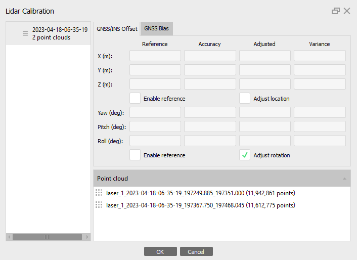
Click OK button.
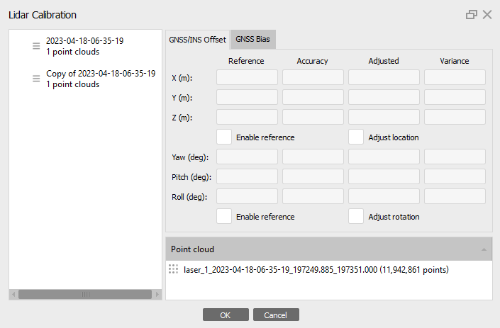
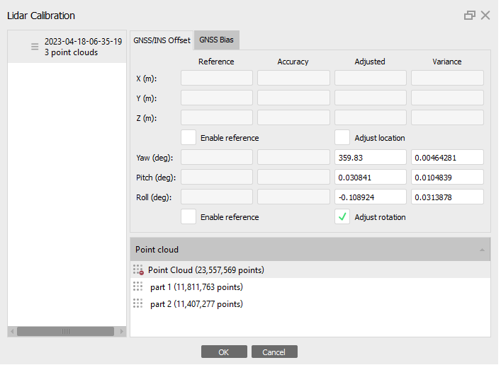
Only one set of displacement parameters can be associated with a trajectory. If different displacement parameters need to be applied to several point clouds associated with the same trajectory, then the trajectory will have to be duplicated for each set of offsets. To duplicate the trajectory file, select the appropriate command in the context menu and assign different trajectory files for each point cloud. Then the 2 parts will be displayed in the Lidar Calibration dialog box:
To calculate the values, you need to perform an alignment. Select Workflow > Align Laser Scans. Set Accuracy for alignment and it is important to enable the Use initial orientation option as in the screenshot below:

- Accuracy - at High accuracy setting the software works with the original distance between points, Medium setting causes downscaling by factor of 4, at Low accuracy source files are downscaled by factor of 16, and Lowest value means further downscaling by 4 times more. Highest accuracy setting upscales the distance between points by factor of 4.
- Reset current alignment - if this option is enebled, all the key, and matching points will be discarded and the alignment procedure will be started from the very beginning. Uncheck this option to sub align some extra laser scans added to the chunk with already aligned set of laser scans.
- Key point limit - the number indicates upper limit of feature points on every laser scans to be taken into account during current processing stage. Using zero value allows Metashape to find as many key points as possible, but it may result in a big number of less reliable points.
- Vertical axis - set the vertical axis (X, Y or Z) of rotation of the laser scan.
- Use initial orientation - parameter allows to improve the result of key points matching based on the available orientation of the aerolidars.
You do not need to use the Reset current alignment option, because we will refine the values based on the aligned data. And it is also important to enable the Reuse local frame option to improve the alignment of aerolidars.
Click OK button to start the alignment process. The calculated values will be available in the Lidar Calibration dialog window after alignment (select Tools > Lidar Calibration):
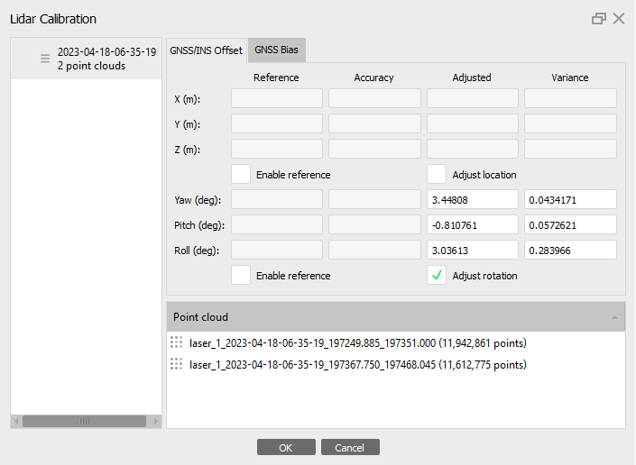
The result after alignment in the Model view:

One Point Cloud Combined in Third-Party Software and One Trajectory File
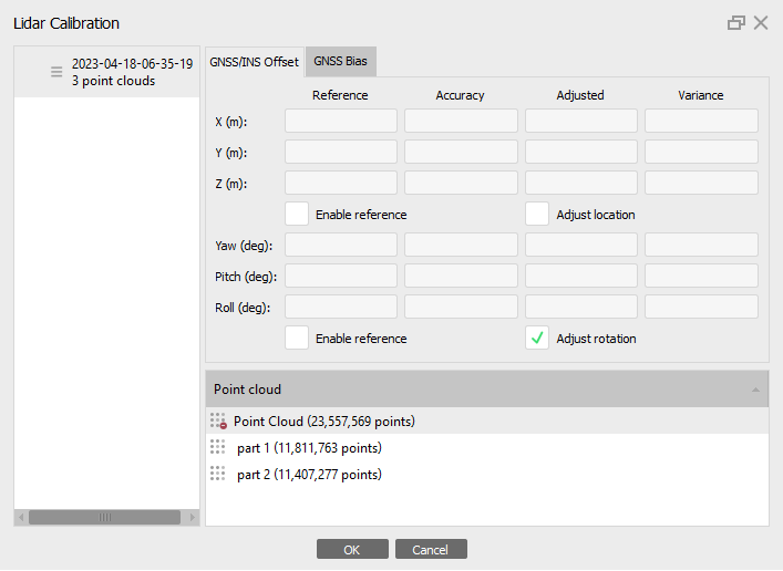
There are cases when point clouds were combined in a third-party program and imported to the Metashape as one cloud, but there are irregularities at route crossing. In this case, using the trajectory masking tool, you need to divide the point cloud into several parts.

Then disable the original point cloud so that it is not taken into account. Selects Disable Laser Scans option from the LiDAR context menu on the Workspace pane.
Enable the Adjust rotation option in the Lidar Calibration dialog window. Select Tools > LiDAR Calibration:
To calculate the values, you need to perform an alignment. Select Workflow > Align Laser Scans:

The calculated values will be available in the Lidar Calibration dialog window after alignment (select Tools > Lidar Calibration):
GNSS Bias
A systematic shift may occur between the coordinate system of the LiDAR point cloud and the coordinate system of the reference data (ground control points). This could be noticed through inspection of the values on the Error tab of the Reference pane. This discrepancy in the data caused by GNSS bias should be corrected for quality processing outputs. The linear values of this shift can be calculated and corrected directly in Metashape.
To perform the correction, it is important that the project has GCPs and their positions are refined manually on the point cloud - when a marker position has been refined by the user, the marker is displayed in green.
We thank Vertical Aspect for providing the data used in this and the next sections. The original LiDAR point cloud was manually pre-shifted to simulate project situation where the GNSS Bias tool is recommended for proper processing of the data.
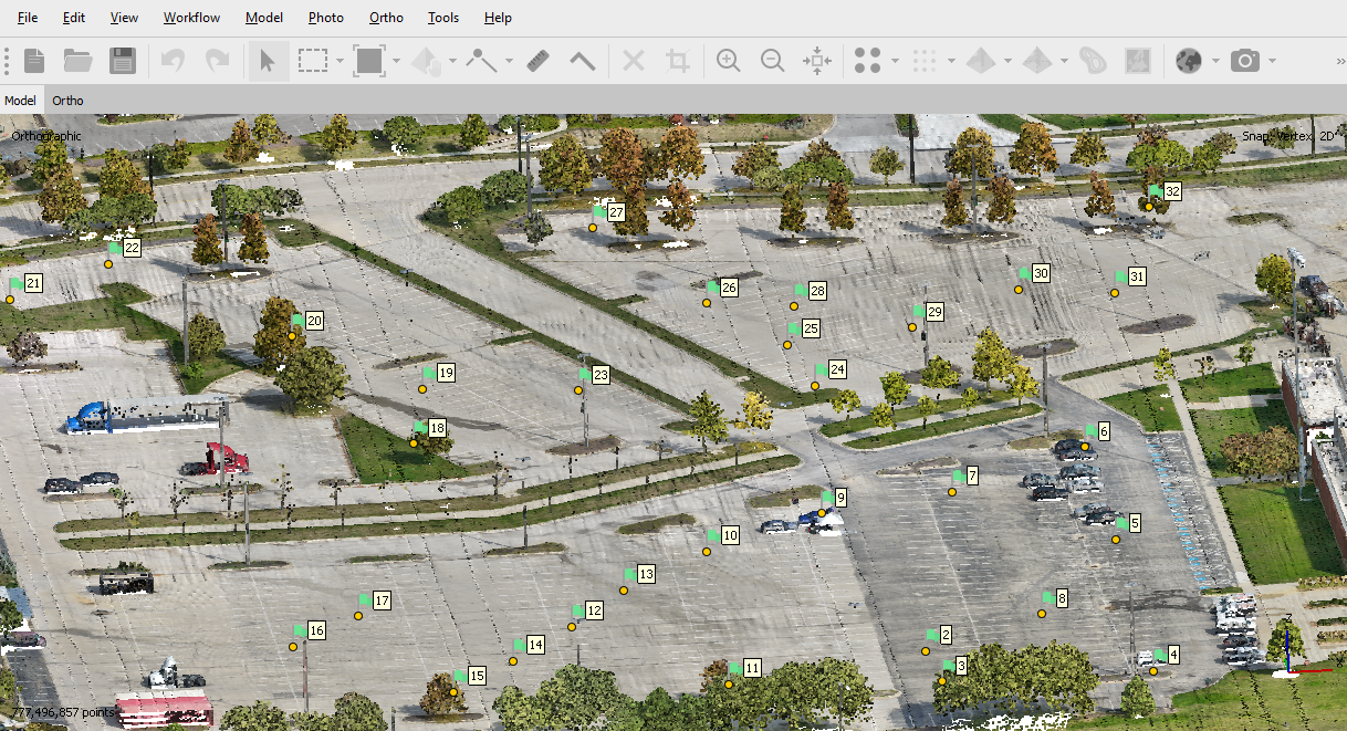
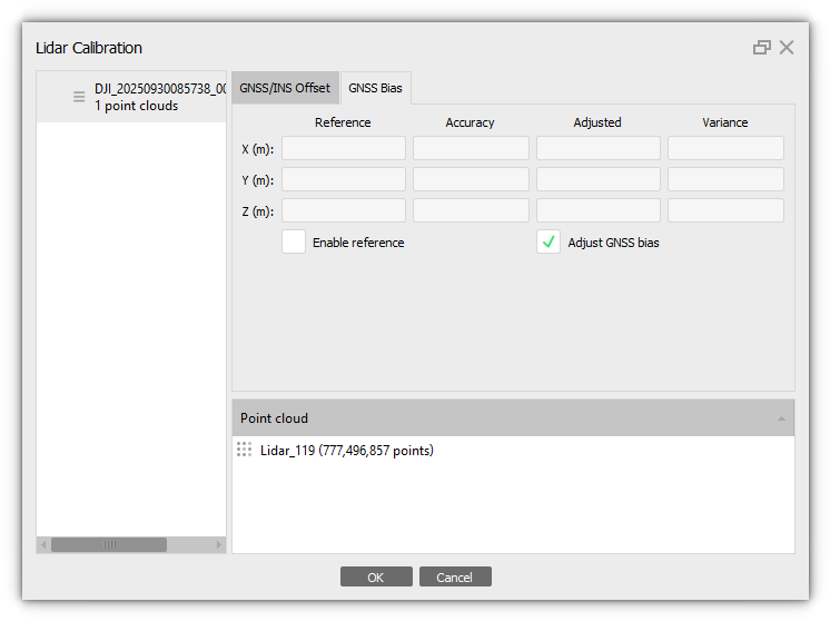
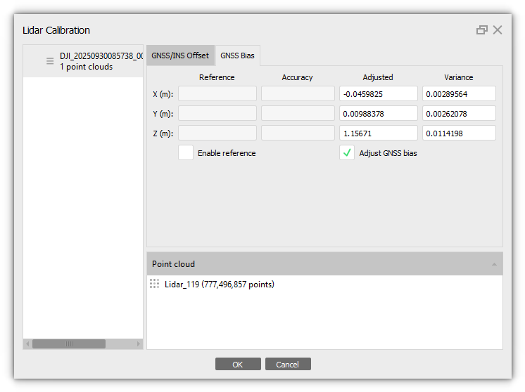
To calculate and minimize this error, enable Adjust GNSS bias on the GNSS Bias tab of the LiDAR Calibration dialog box (select Tools > Lidar Calibration) before alignment:
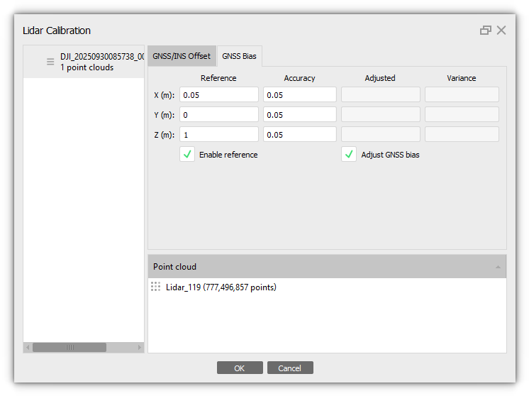
If these offsets are known, they should be input into Metashape before alignment. In this case also turn on the checkbox for the Enable reference option along with enabling Adjust GNSS bias option:
If the project aims at processing of lidar and photogrammetry data together, you should enable the Match depth maps option for the laser scans alignment processing step (the algorithm combines together depth maps from photogrammetry data and points from the LiDAR point cloud):Before alignment, in this scenario it is also recommended to clarify the positions of the markers on the images not only on the point cloud itself. Then marker projections on the images are also used in LiDAR Bias values calculation, which adds to the accuracy of the adjustment.
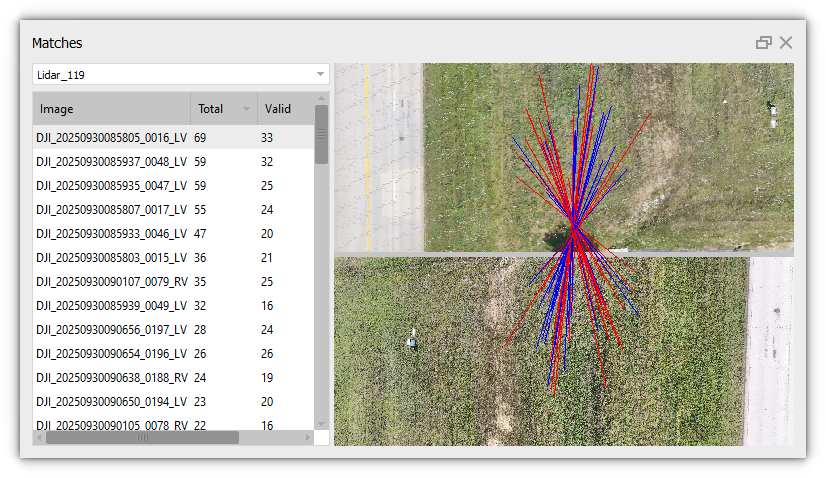
To make sure that photogrammetry data and lidar points were properly matched, valid matches can be checked through the Matches dialog window (select View Matches... option from the images context menu):
After alignment the adjusted values of the GNS offset can be viewed in Lidar Calibration dialog:
Measure Elevation
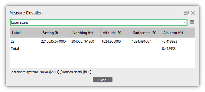
The Measure Elevation tool helps estimate the altitude error of lidar points source reference data against control and check points source reference data, which is usually more precise. The dialog box will display difference between altitude values for the original marker position (imported into the project) and the altitude values for the marker position specified manually on the LiDAR point cloud.
To calculate this value, select the Measure Elevation command from the markers' context menu on the Reference pane:
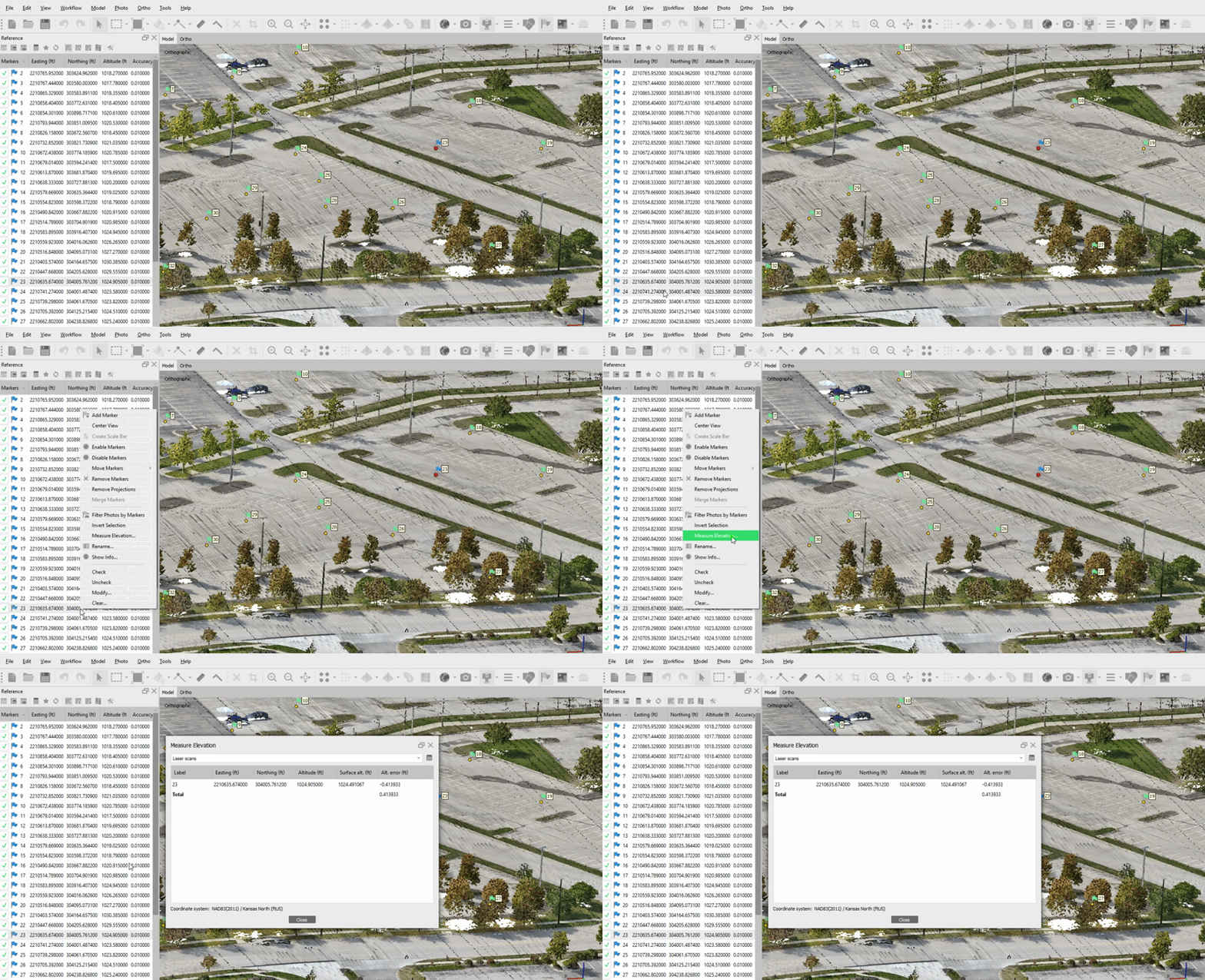
Values are calculated for the markers selected in the Reference pane. If you need to calculate the value for all markers, select them all on the Reference pane, and then use the tool.
The Surface alt. (m) column displays the altitude value of the marker on the selected surface, in our example, on the "surface" of the laser scan:
Difference View
To evaluate the accuracy of the alignment of LiDAR data sets, the Accuracy View tool has been added. Tool displays the area of overlap of LiDAR point clouds and query the points according to the error value. The error value is calculated as the distance from a point in one cloud to the averaged plane defined by the neighborhood of the corresponding point in the other LiDAR point cloud.
Select the appropriate tool on the Toolbar (Show Laser Scans > Difference View):

IMPORTANT: When using this tool, the Model view doesn't display the original point clouds. Instead, it displays the clouds with calculated errors for accuracy assessment. These areas cannot be edited, and the Selection tools are not available for them.
The legend displays the error value and is calculated for each project separately. The points are colored according to the error values (distances) in this area. Blue represents the smallest error, while red represents the largest error:

If you want to calculate error values for a specific area, you need to select this area first (using the selection tools on the Toolbar):

And then use the Difference View tool:
